Fifteen weeks. Three labs. Two paper presentations. One team project that ended in a null result I’m still proud of.
EE 599: Robotic Mobility, taught by Prof. Feifei Qian in Fall 2025, was the most hands-on course I took at USC — and the one that most changed how I think. Not just about robots. About what it means to know something: to have the math, the hardware, and the measurement all agree with each other, and to notice when they don’t.
This is the full retrospective: the labs, the project, the teaching, and what stuck.
The shape of it
Looking back, three ideas ran underneath the whole semester, and I only saw the pattern clearly when I wrote my study guide at the end: template-based control (parameterized clocks that generate gaits), geometric mechanics (shape-space geometry that predicts and optimizes motion), and dynamic locomotion (energy exchange and stability analysis). Everything I learned was one of those three wearing different clothes.
The rhythm that made it stick: watch the thing move, build the physical picture, write the math, then test it on hardware. Every unit followed that order. It’s the order I still use when I’m learning something hard.
Lab 1: learning to speak servo
The first lab put a Buehler clock in my hands — or rather, in my servos.
The setup: a small quadruped, four Dynamixel-class servos, and a controller that generates leg trajectories from a handful of parameters — stride period, duty cycle, phase offsets between legs. Lab 1 was about learning to command a servo properly: position mode, velocity mode, torque mode, and what the motor is actually doing under each.
I came out of it with plots I still keep: per-joint traces of commanded angle, measured velocity, and estimated torque across gait cycles. The unglamorous kind of data. But it was the first time I’d measured a gait instead of just watching one, and it taught me the habit the whole course kept reinforcing: the plot is the truth; the theory is the hypothesis.
The conceptual payload of Lab 1 was small but load-bearing: a gait is not a script of joint angles. It’s a parameterized clock. Change the phase offset between the rear pair and the front pair and you’ve changed the gait — same hardware, same code, different animal. That idea — behavior as a point in parameter space — is the seed everything else grew from.
Lab 2: the gait playground
Lab 2 was the playground: the same quadruped, but now the task was to explore the gait parameter space systematically. Phase relationships between leg pairs, duty cycle sweeps, the transition from walking to bounding.
Bounding was the revelation. Offset the rear pair by half a cycle from the front pair and the little quadruped stops walking and starts bounding — front legs and rear legs moving as pairs, the body pitching with each stride. It’s the gait cats use at speed, and it falls out of one parameter. I spent a long time just watching it, changing the number by a tenth and watching the behavior reorganize.
The lesson wasn’t “bounding exists.” The lesson was that coordination is a continuous space, not a menu of options. Walking, trotting, bounding — they’re neighborhoods in the same parameter space, and the boundaries between them are where the interesting physics lives.
Lab 3: geometric mechanics, or the week the math got beautiful
Lab 3 was the intellectual center of the course, and the hardest thing I’d done at USC to that point.
The robot: a three-link kinematic snake, two servos, moving on a surface. The question: given that you can only control the two joint angles, what joint trajectories produce the most forward motion — or the most rotation — per cycle?
The answer comes from geometric mechanics, and it’s one of the most beautiful ideas in robotics: your joints live in shape space (the space of α₁, α₂), your body lives in the world, and the map between joint velocity and body velocity is a connection. The net displacement from one gait cycle is the line integral of that connection around the loop your joints trace — and by Stokes’ theorem, that equals the surface integral of the curl of the connection over the area the loop encloses.
In plain language: to move forward, draw a loop in joint space that encloses as much positive curl as possible. The curl field is called the height function, and once you plot it, gait design becomes a visual, almost artistic act: find the bright regions, draw your loop around them.
I computed the connection fields for the 3-link snake (the denominator D = sin(α₁) − sin(α₂) + sin(α₁ − α₂), with singularities masked where it vanishes), plotted the height functions Hₓ and Hθ, and designed three gaits as circles in shape space:
- Forward, minimal rotation: center (−0.090, 0.045) rad, counterclockwise — sits in the strong positive Hₓ region while dodging high-Hθ zones
- Max counterclockwise rotation: center (0.765, 0.900) rad
- Max clockwise rotation: center (−0.900, −0.765) rad — the geometric mirror of the second
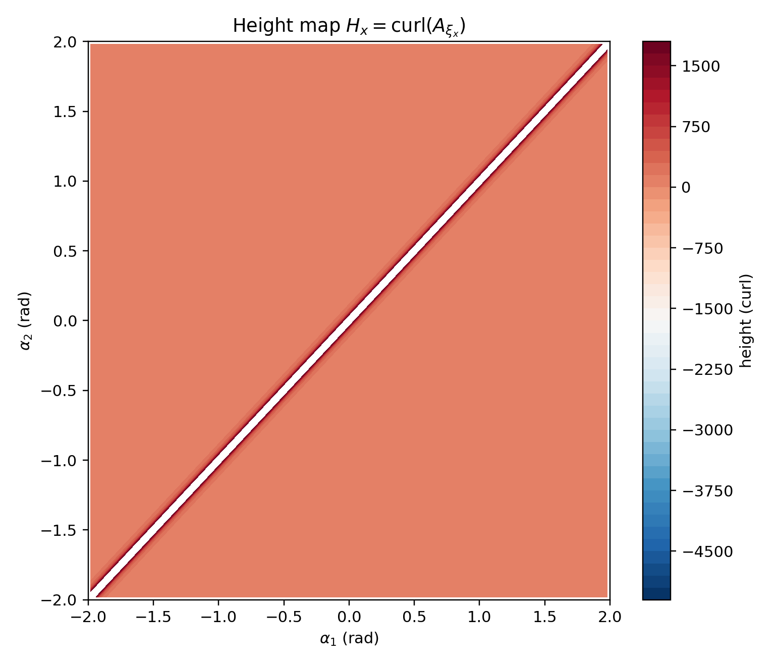 The Hx height function: bright regions are where a gait loop harvests the most forward motion per cycle. Gait design becomes drawing loops around the bright spots.
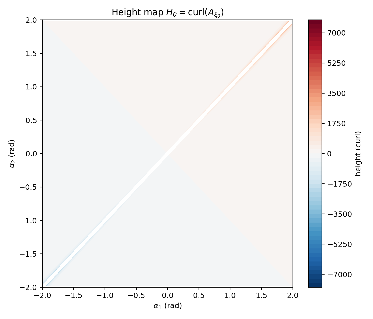 The Htheta landscape: mirror-symmetric about the origin — which is why the two rotation gaits are geometric mirrors of each other.
Then the lab asked the questions that turned computation into understanding. Is a circle optimal? (No — an ellipse aligned to the height-function ridge, or a contour-following path, encloses more curl per unit perimeter; circles are just the practical compromise.) Does the starting shape matter? (Net displacement per cycle: no — Stokes’ theorem doesn’t care where on the loop you start. World-frame trajectory: yes — like steering a car the same way from different initial headings.)
And then Task 4: take the gaits to hardware. Run the physical snake, measure actual displacement per cycle, and fill in the predicted-vs-measured comparison table. The course never let the math live alone. Every beautiful integral had to survive contact with a servo.
The Lab 3 snake running one of the designed gaits on the bench — the connection vector fields, made flesh (well, LEGO).
Learning to read papers
Somewhere in the middle of the semester I had to stand up and explain two research papers in ten minutes each, to people who’d read the same papers. That teaches you something no amount of reading does: you have to decide what the paper’s one idea is, and defend that choice out loud. It’s the conference-talk skill, compressed — and it’s changed how I read everything since.
Walking is a pendulum, running is a spring
The dynamics units gave me the vocabulary I still use. Walking is an inverted pendulum: the body’s center of mass vaults over a stiff leg, trading kinetic energy for gravitational potential energy and back. The rimless wheel model — a wheel with spokes but no rim, each spoke a step — captures it with shocking economy. Stability analysis via Poincaré maps and cobweb diagrams: does the gait converge back to itself after a perturbation, or fall over?
Running is a spring. The spring-loaded inverted pendulum (SLIP): the leg compresses on touchdown, stores energy, releases it at liftoff. Same center-of-mass curves as walking, reversed mechanism — gravity doing the work in one, the spring in the other.
What made it land wasn’t the equations alone — it was seeing them from someone who’d built the machines they described. The math stopped being abstract the moment it had a robot attached.
Terrain: where the course pointed at the project
The last lecture units — terrain adaptation on deformable and rough terrain — were the on-ramp to the final project. Granular media: how sand flows around an intruder, resistive force theory (RFT) for predicting forces on legs moving through grains, sidewinding on sand inclines, sand-swimming. The message: everything you learned about gaits assumed a rigid world. The real world deforms, and the physics changes.
My team took that message literally. Our project asked whether timed vibration — fluidizing the sand during leg swing, letting it compact during stance — could improve locomotion efficiency on granular media. Ten weeks, biweekly checkpoints, a bead testbed, current sensing, and a final report written like a conference paper.
The result was a null: cost of transport went from 50 to 77 once we honestly accounted for the vibration motors’ power draw. I’ve written the full story separately — the deep dive is here. What the semester gave me for that project wasn’t the idea — it was the habits: keep a predicted-vs-measured table, report the null instead of hiding it. Be wrong in public, carefully.
What stuck
A year later, here’s what I actually kept:
Motion is geometry before it’s force. Lab 3 rewired me. When I see a periodic system now — a gait, a switching converter, a control loop — I think in terms of loops in parameter space and what they enclose. That picture has leaked into everything.
Measure the thing you claim. Lab 1’s torque plots, Lab 3’s predicted-vs-measured tables, the project’s current sensor on the vibration rail — the course graded the comparison between theory and hardware, not the theory alone. My line about being “the person who notices when a metric lies about a signal” was born here, in the gap between a CoT of 49 and a CoT of 77.
Derive it yourself. The no-AI policy felt strict in week 2 and felt like a gift by week 10. The connection fields, the height functions, the gait centers — I can still reconstruct them because I built them by hand. Fluency isn’t having the answer; it’s having the path to the answer.
Research is a format, not a talent. Proposal, checkpoints, demo, conference-style report — the project taught the motions of research: hypothesis, experiment plan, preliminary data, honest discussion. You don’t need permission to do science; you need a lab notebook and a deadline.
Learn in the right order. Watch it move → build the physical picture → write the math → test it. I keep catching myself reversing that order on new topics — reaching for equations before I have a picture — and the picture-first version wins every time.
The quadruped from Labs 1–2 and the final project now lives on my projects page, with photos and video from the bead testbed. The full project writeup — hypothesis, firmware, and the honest null result — is here.