<?xml version="1.0" encoding="utf-8"?><feed xmlns="http://www.w3.org/2005/Atom" ><generator uri="https://jekyllrb.com/" version="3.10.0">Jekyll</generator><link href="https://visareve.github.io/feed.xml" rel="self" type="application/atom+xml" /><link href="https://visareve.github.io/" rel="alternate" type="text/html" /><updated>2026-09-26T16:30:52-07:00</updated><id>https://visareve.github.io/feed.xml</id><title type="html">Vi Sa Re Ve</title><subtitle>Vidya Sagar Reddy Venna (Vi Sa Re Ve) — ML engineer working on biosignals, neural decoding, and time-series ML. MS ECE (ML &amp; Data Science) at USC, May 2026.</subtitle><author><name>Vidya Sagar Reddy Venna</name><email>vvenna@usc.edu</email></author><entry><title type="html">What EE 599 Actually Taught Me: A Semester of Robotic Mobility</title><link href="https://visareve.github.io/posts/ee599-robotic-mobility/" rel="alternate" type="text/html" title="What EE 599 Actually Taught Me: A Semester of Robotic Mobility" /><published>2026-09-26T00:00:00-07:00</published><updated>2026-09-26T00:00:00-07:00</updated><id>https://visareve.github.io/posts/ee599-robotic-mobility</id><content type="html" xml:base="https://visareve.github.io/posts/ee599-robotic-mobility/"><![CDATA[<p>Fifteen weeks. Three labs. Two paper presentations. One team project that ended in a null result I’m still proud of.</p>

<p>EE 599: Robotic Mobility, taught by Prof. Feifei Qian in Fall 2025, was the most hands-on course I took at USC — and the one that most changed how I think. Not just about robots. About what it means to <em>know</em> something: to have the math, the hardware, and the measurement all agree with each other, and to notice when they don’t.</p>

<p>This is the full retrospective: the labs, the project, the teaching, and what stuck.</p>

<h2 id="the-shape-of-it">The shape of it</h2>

<p>Looking back, three ideas ran underneath the whole semester, and I only saw the pattern clearly when I wrote my study guide at the end: <strong>template-based control</strong> (parameterized clocks that generate gaits), <strong>geometric mechanics</strong> (shape-space geometry that predicts and optimizes motion), and <strong>dynamic locomotion</strong> (energy exchange and stability analysis). Everything I learned was one of those three wearing different clothes.</p>

<p>The rhythm that made it stick: watch the thing move, build the physical picture, write the math, then test it on hardware. Every unit followed that order. It’s the order I still use when I’m learning something hard.</p>

<h2 id="lab-1-learning-to-speak-servo">Lab 1: learning to speak servo</h2>

<p>The first lab put a Buehler clock in my hands — or rather, in my servos.</p>

<p>The setup: a small quadruped, four Dynamixel-class servos, and a controller that generates leg trajectories from a handful of parameters — stride period, duty cycle, phase offsets between legs. Lab 1 was about learning to command a servo properly: position mode, velocity mode, torque mode, and what the motor is actually doing under each.</p>

<p>I came out of it with plots I still keep: per-joint traces of commanded angle, measured velocity, and estimated torque across gait cycles. The unglamorous kind of data. But it was the first time I’d <em>measured</em> a gait instead of just watching one, and it taught me the habit the whole course kept reinforcing: <strong>the plot is the truth; the theory is the hypothesis.</strong></p>

<p>The conceptual payload of Lab 1 was small but load-bearing: a gait is not a script of joint angles. It’s a <em>parameterized clock</em>. Change the phase offset between the rear pair and the front pair and you’ve changed the gait — same hardware, same code, different animal. That idea — behavior as a point in parameter space — is the seed everything else grew from.</p>

<h2 id="lab-2-the-gait-playground">Lab 2: the gait playground</h2>

<p>Lab 2 was the playground: the same quadruped, but now the task was to explore the gait parameter space systematically. Phase relationships between leg pairs, duty cycle sweeps, the transition from walking to bounding.</p>

<p>Bounding was the revelation. Offset the rear pair by half a cycle from the front pair and the little quadruped stops walking and starts <em>bounding</em> — front legs and rear legs moving as pairs, the body pitching with each stride. It’s the gait cats use at speed, and it falls out of one parameter. I spent a long time just watching it, changing the number by a tenth and watching the behavior reorganize.</p>

<p>The lesson wasn’t “bounding exists.” The lesson was that <strong>coordination is a continuous space, not a menu of options.</strong> Walking, trotting, bounding — they’re neighborhoods in the same parameter space, and the boundaries between them are where the interesting physics lives.</p>

<h2 id="lab-3-geometric-mechanics-or-the-week-the-math-got-beautiful">Lab 3: geometric mechanics, or the week the math got beautiful</h2>

<p>Lab 3 was the intellectual center of the course, and the hardest thing I’d done at USC to that point.</p>

<p>The robot: a three-link kinematic snake, two servos, moving on a surface. The question: given that you can only control the two joint angles, what joint trajectories produce the most forward motion — or the most rotation — per cycle?</p>

<p>The answer comes from <strong>geometric mechanics</strong>, and it’s one of the most beautiful ideas in robotics: your joints live in <em>shape space</em> (the space of α₁, α₂), your body lives in the world, and the map between joint velocity and body velocity is a <em>connection</em>. The net displacement from one gait cycle is the line integral of that connection around the loop your joints trace — and by Stokes’ theorem, that equals the <em>surface integral of the curl</em> of the connection over the area the loop encloses.</p>

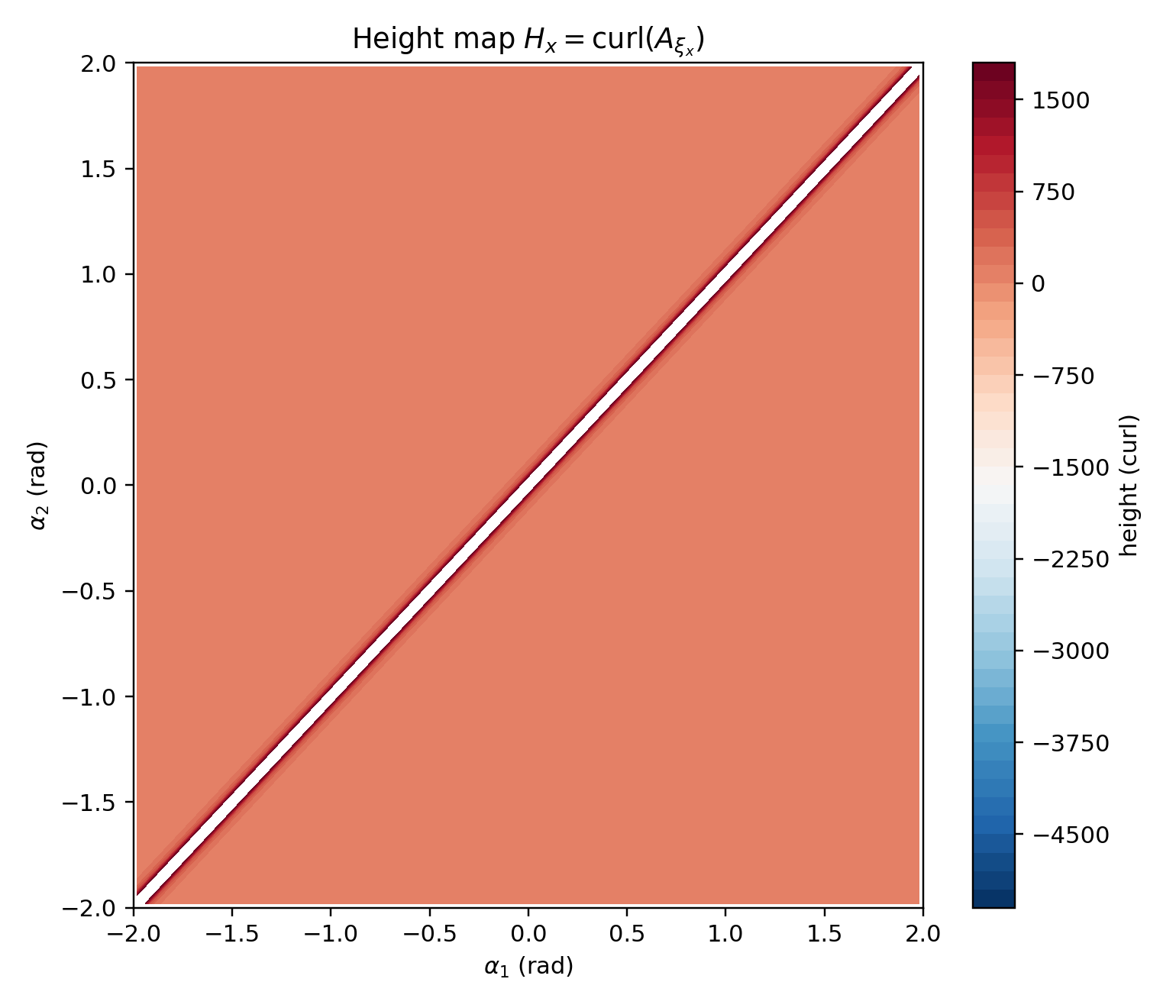
<p>In plain language: <strong>to move forward, draw a loop in joint space that encloses as much positive curl as possible.</strong> The curl field is called the <em>height function</em>, and once you plot it, gait design becomes a visual, almost artistic act: find the bright regions, draw your loop around them.</p>

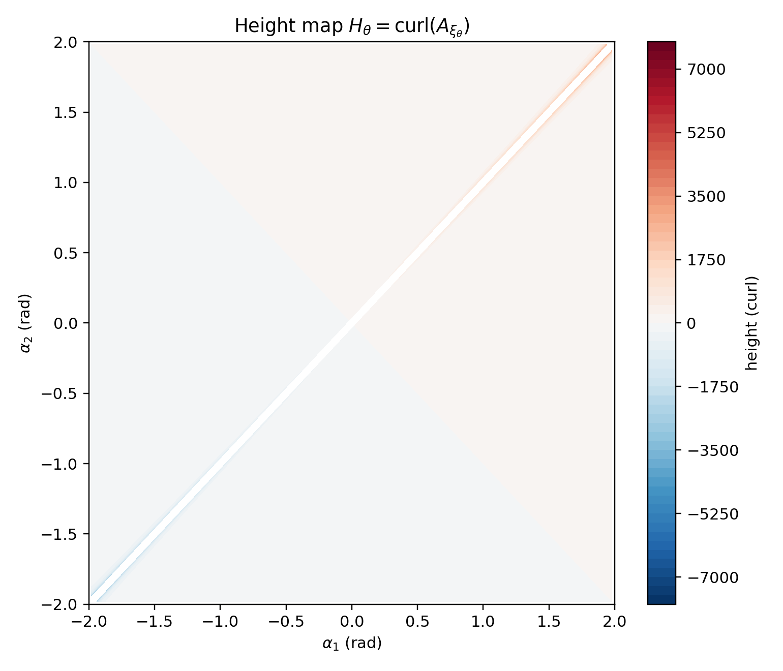
<p>I computed the connection fields for the 3-link snake (the denominator D = sin(α₁) − sin(α₂) + sin(α₁ − α₂), with singularities masked where it vanishes), plotted the height functions Hₓ and Hθ, and designed three gaits as circles in shape space:</p>

<ul>
  <li><strong>Forward, minimal rotation:</strong> center (−0.090, 0.045) rad, counterclockwise — sits in the strong positive Hₓ region while dodging high-Hθ zones</li>
  <li><strong>Max counterclockwise rotation:</strong> center (0.765, 0.900) rad</li>
  <li><strong>Max clockwise rotation:</strong> center (−0.900, −0.765) rad — the geometric mirror of the second</li>
</ul>

<p><img src="/assets/img/course/ee599/height-Hx.png" alt="Height function Hx — forward displacement harvested per unit area of shape space" />
<em>The Hx height function: bright regions are where a gait loop harvests the most forward motion per cycle. Gait design becomes drawing loops around the bright spots.</em></p>

<p><img src="/assets/img/course/ee599/height-Htheta.png" alt="Height function Htheta — rotation harvested per unit area of shape space" />
<em>The Htheta landscape: mirror-symmetric about the origin — which is why the two rotation gaits are geometric mirrors of each other.</em></p>

<p>Then the lab asked the questions that turned computation into understanding. <em>Is a circle optimal?</em> (No — an ellipse aligned to the height-function ridge, or a contour-following path, encloses more curl per unit perimeter; circles are just the practical compromise.) <em>Does the starting shape matter?</em> (Net displacement per cycle: no — Stokes’ theorem doesn’t care where on the loop you start. World-frame trajectory: yes — like steering a car the same way from different initial headings.)</p>

<p>And then Task 4: take the gaits to hardware. Run the physical snake, measure actual displacement per cycle, and fill in the predicted-vs-measured comparison table. The course never let the math live alone. <strong>Every beautiful integral had to survive contact with a servo.</strong></p>

<video controls="" preload="metadata" style="width:100%; border-radius:8px;" src="/assets/vid/course/ee599/snake-gait.mp4"></video>
<p><em>The Lab 3 snake running one of the designed gaits on the bench — the connection vector fields, made flesh (well, LEGO).</em></p>

<h2 id="learning-to-read-papers">Learning to read papers</h2>

<p>Somewhere in the middle of the semester I had to stand up and explain two research papers in ten minutes each, to people who’d read the same papers. That teaches you something no amount of reading does: you have to decide what the paper’s <em>one</em> idea is, and defend that choice out loud. It’s the conference-talk skill, compressed — and it’s changed how I read everything since.</p>

<h2 id="walking-is-a-pendulum-running-is-a-spring">Walking is a pendulum, running is a spring</h2>

<p>The dynamics units gave me the vocabulary I still use. <strong>Walking is an inverted pendulum</strong>: the body’s center of mass vaults over a stiff leg, trading kinetic energy for gravitational potential energy and back. The rimless wheel model — a wheel with spokes but no rim, each spoke a step — captures it with shocking economy. Stability analysis via Poincaré maps and cobweb diagrams: does the gait converge back to itself after a perturbation, or fall over?</p>

<p><strong>Running is a spring.</strong> The spring-loaded inverted pendulum (SLIP): the leg compresses on touchdown, stores energy, releases it at liftoff. Same center-of-mass curves as walking, reversed mechanism — gravity doing the work in one, the spring in the other.</p>

<p>What made it land wasn’t the equations alone — it was seeing them from someone who’d <em>built</em> the machines they described. The math stopped being abstract the moment it had a robot attached.</p>

<h2 id="terrain-where-the-course-pointed-at-the-project">Terrain: where the course pointed at the project</h2>

<p>The last lecture units — terrain adaptation on deformable and rough terrain — were the on-ramp to the final project. Granular media: how sand flows around an intruder, resistive force theory (RFT) for predicting forces on legs moving through grains, sidewinding on sand inclines, sand-swimming. The message: everything you learned about gaits assumed a rigid world. The real world deforms, and the physics changes.</p>

<p>My team took that message literally. Our project asked whether timed vibration — fluidizing the sand during leg swing, letting it compact during stance — could improve locomotion efficiency on granular media. Ten weeks, biweekly checkpoints, a bead testbed, current sensing, and a final report written like a conference paper.</p>

<p>The result was a null: cost of transport went from 50 to 77 once we honestly accounted for the vibration motors’ power draw. I’ve written the full story separately — <a href="/2026/09/26/timed-vibration-granular-locomotion/">the deep dive is here</a>. What the semester gave me for that project wasn’t the idea — it was the habits: keep a predicted-vs-measured table, report the null instead of hiding it. <strong>Be wrong in public, carefully.</strong></p>

<h2 id="what-stuck">What stuck</h2>

<p>A year later, here’s what I actually kept:</p>

<p><strong>Motion is geometry before it’s force.</strong> Lab 3 rewired me. When I see a periodic system now — a gait, a switching converter, a control loop — I think in terms of loops in parameter space and what they enclose. That picture has leaked into everything.</p>

<p><strong>Measure the thing you claim.</strong> Lab 1’s torque plots, Lab 3’s predicted-vs-measured tables, the project’s current sensor on the vibration rail — the course graded the comparison between theory and hardware, not the theory alone. My line about being “the person who notices when a metric lies about a signal” was born here, in the gap between a CoT of 49 and a CoT of 77.</p>

<p><strong>Derive it yourself.</strong> The no-AI policy felt strict in week 2 and felt like a gift by week 10. The connection fields, the height functions, the gait centers — I can still reconstruct them because I built them by hand. Fluency isn’t having the answer; it’s having the path to the answer.</p>

<p><strong>Research is a format, not a talent.</strong> Proposal, checkpoints, demo, conference-style report — the project taught the <em>motions</em> of research: hypothesis, experiment plan, preliminary data, honest discussion. You don’t need permission to do science; you need a lab notebook and a deadline.</p>

<p><strong>Learn in the right order.</strong> Watch it move → build the physical picture → write the math → test it. I keep catching myself reversing that order on new topics — reaching for equations before I have a picture — and the picture-first version wins every time.</p>

<hr />

<p><em>The quadruped from Labs 1–2 and the final project now lives on <a href="/projects/quadruped/">my projects page</a>, with photos and video from the bead testbed. The full project writeup — hypothesis, firmware, and the honest null result — is <a href="/2026/09/26/timed-vibration-granular-locomotion/">here</a>.</em></p>]]></content><author><name>Vidya Sagar Reddy Venna</name><email>vvenna@usc.edu</email></author><category term="robotics" /><category term="course-notes" /><category term="robotics" /><category term="locomotion" /><category term="geometric-mechanics" /><category term="terradynamics" /><summary type="html"><![CDATA[Fifteen weeks, three labs, one honest null result — what a semester of legged locomotion taught me about motion, measurement, and teaching.]]></summary><media:thumbnail xmlns:media="http://search.yahoo.com/mrss/" url="https://visareve.github.io/assets/img/og-card.png" /><media:content medium="image" url="https://visareve.github.io/assets/img/og-card.png" xmlns:media="http://search.yahoo.com/mrss/" /></entry><entry><title type="html">Timed Vibration on Granular Media: A Null Result, Told With Numbers</title><link href="https://visareve.github.io/posts/timed-vibration-granular-locomotion/" rel="alternate" type="text/html" title="Timed Vibration on Granular Media: A Null Result, Told With Numbers" /><published>2026-09-26T00:00:00-07:00</published><updated>2026-09-26T00:00:00-07:00</updated><id>https://visareve.github.io/posts/timed-vibration-granular-locomotion</id><content type="html" xml:base="https://visareve.github.io/posts/timed-vibration-granular-locomotion/"><![CDATA[<p>Sand is the only terrain I know that can’t decide what it is. Step on it right and it’s concrete. Step on it wrong and it’s soup. For our EE 579 final project, my team asked: what if a robot could flip that switch on purpose — fluidize the ground for the leg that’s swinging forward, then let it jam solid for the leg that’s pushing off? All inside a single stride.</p>

<p>We built it. We measured it. It didn’t work. This is the honest version, with numbers.</p>

<video controls="" playsinline="" preload="metadata" poster="/assets/img/quadruped/granular-walk-poster.jpg" style="width:100%;">
  <source src="/assets/vid/quadruped/granular-walk.mp4" type="video/mp4" />
  Your browser does not support embedded video.
</video>
<p><em>Full test run on the granular testbed — the bounding gait carrying the quadruped across the bead bed.</em></p>

<h2 id="the-bet">The bet</h2>

<p>Legged locomotion on granular media has a clean piece of physics behind it, from Li, Umbanhowar, Komsuoglu, and Goldman: on dense, packed sand a legged robot does efficient “rotary walking”; on loose, fluid-like sand the same robot degrades into “swimming” — lots of motion, no progress. The substrate’s state is the whole game.</p>

<p>Two more facts from the literature made the bet tempting:</p>

<ol>
  <li><strong>Vibration fluidizes.</strong> Marston et al. showed a vibrating object penetrates sand with dramatically reduced resistance — the grains lose their force chains and flow.</li>
  <li><strong>Vibration compacts — after the fact.</strong> Stop shaking a box of grains and they settle denser and stronger than before (Raihane et al. and others). The aftermath of vibration is a firmer packing.</li>
</ol>

<p>Nobody had combined the two into one gait cycle: shake during swing (low drag for the recovering leg), stop during stance (firm foothold for the pushing leg). Timed, intermittent, synchronized to the stride. Our research question: can a legged robot improve locomotor efficiency by cyclically switching the sand between fluid and solid in sync with its gait?</p>

<h2 id="the-machine">The machine</h2>

<p>Four Dynamixel XL-320 servos, one degree of freedom per leg, on a rigid chassis. The gait is a Buehler clock — the standard trick for legged robots: each stride splits into a slow phase (stance, on the ground) and a fast phase (swing, in the air), set by the slow-phase extent, a phase offset, a duty cycle, and the stride period. Ours ran a bounding gait — front pair and rear pair half a period apart, 4-second period, 0.56 duty cycle.</p>

<p>The vibration system: six 14 mm coin motors — the kind that buzz in a phone — under the chassis, driven by two Adafruit DRV2605L haptic controllers (front pair on hardware I2C, rear pair on bit-banged software I2C, because of course we ran out of hardware buses). An Arduino orchestrated everything: legs in swing → vibrate; touchdown → keep vibrating 500 ms into stance to help the foot settle, then cut it.</p>

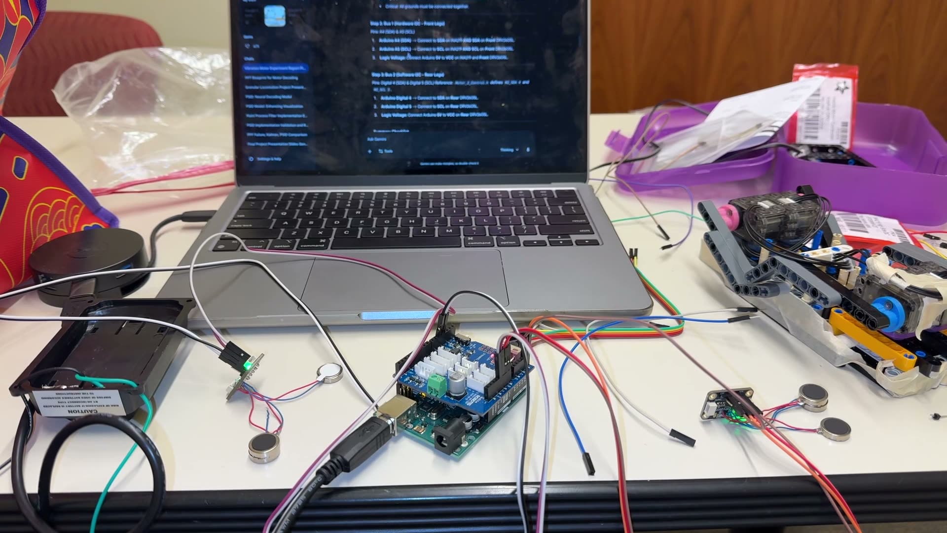
<p><img src="/assets/img/quadruped/workbench.jpg" alt="The vibration rig mid-build — Arduino, driver shield, coin motors, wiring doc on the laptop" />
<em>The rig on the workbench: Arduino with the driver shield, coin vibration motors scattered around, and the DRV2605L wiring notes open on the laptop.</em></p>
<p>The part I’m proudest of isn’t the idea, it’s the instrumentation. The XL-320s report present load, so every 20 ms the firmware logged per-leg torque (load × stall torque) and mechanical power (torque × angular velocity), streaming tab-separated telemetry at 115200 baud. Plus the unglamorous hack the project needed: the XL-320 only positions over 0–300°, so when the Buehler clock commanded an angle inside the dead zone, the firmware flipped that servo to velocity mode, coasted through, and flipped back. Robots are 10% inspiration, 90% dead-zone handling.</p>

<p>The course built toward this honestly. Lab 1 was single-servo trajectories — theta vs. time, theta vs. torque plots. Lab 2 was open playground. Lab 3 was the measurement pipeline: the telemetry discipline, displacement tracking, the “how do you know what you claim” part. The final project was all of it at once, with sand.</p>

<h2 id="the-experiment">The experiment</h2>

<p>A wooden box of uniform white beads — macro-scale, spherical, standing in for sand. Zero incline. Cross 2 feet. Control run: bounding gait, no vibration. Experimental run: same gait, timed vibration. Metrics straight from the literature:</p>

<ul>
  <li>Forward velocity, from video timing.</li>
  <li>Per-leg torque and power, from the servo telemetry.</li>
  <li>Cost of transport: <code class="language-plaintext highlighter-rouge">CoT = P / (W * v)</code> — power over weight times velocity. Dimensionless, the standard efficiency score. Lower is better.</li>
</ul>

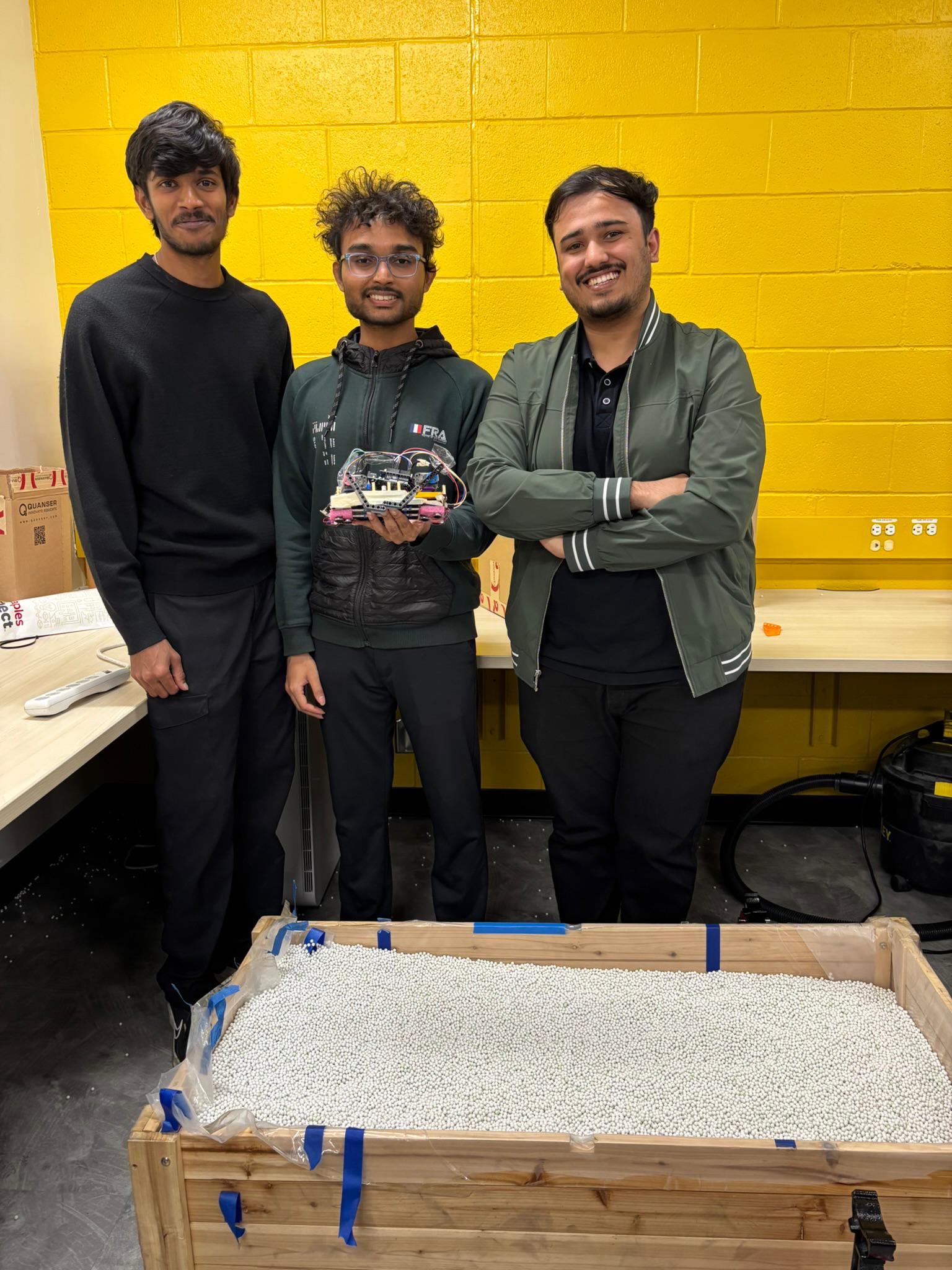
<p><img src="/assets/img/quadruped/team-testbed.jpg" alt="The team with the robot and the granular testbed" />
<em>The testbed: a wooden box of beads standing in for loose terrain.</em></p>

<h2 id="the-numbers">The numbers</h2>

<table>
  <thead>
    <tr>
      <th> </th>
      <th>Control (no vibration)</th>
      <th>Vibration</th>
    </tr>
  </thead>
  <tbody>
    <tr>
      <td>Robot mass</td>
      <td>0.275 kg</td>
      <td>0.325 kg</td>
    </tr>
    <tr>
      <td>Time for 2 ft</td>
      <td>35 s</td>
      <td>42 s</td>
    </tr>
    <tr>
      <td>Leg power</td>
      <td>2.37 W</td>
      <td>2.28 W</td>
    </tr>
    <tr>
      <td>Vibration motor power</td>
      <td>—</td>
      <td>1.3 W (measured, INA219)</td>
    </tr>
    <tr>
      <td>Yield (peak stance) torque</td>
      <td>0.47–0.49 N·m</td>
      <td>0.47 N·m</td>
    </tr>
    <tr>
      <td>Swing drag torque</td>
      <td>0.144 N·m</td>
      <td>0.143 N·m</td>
    </tr>
    <tr>
      <td><strong>Cost of transport</strong></td>
      <td><strong>50</strong></td>
      <td><strong>49 (legs only) → 77 (honest)</strong></td>
    </tr>
  </tbody>
</table>

<p>Read the honest column first. Leg power alone dropped from 2.37 W to 2.28 W — stop there and you’d write “marginal improvement” and move on. That’s the metric lying. The vibration motors drew 1.3 W, measured with an INA219 current sensor — more than half the legs’ power again — and the haptic rig added 50 g to a 275 g robot, an 18% mass penalty before it spent a single joule. Put it all in: CoT 50 → 77. Not a marginal win. A clear loss.</p>

<p>The terrain-interaction numbers back it up: peak stance torque — the ground’s yield force, the foothold quality — didn’t move (0.47–0.49 vs 0.47 N·m). Swing drag didn’t move either (0.144 vs 0.143 N·m). The vibration changed nothing about the sand. It just cost power and weight.</p>

<h2 id="why-it-failed">Why it failed</h2>

<p>A scaling mismatch, and it’s the most useful thing we learned. Our “sand” was macro-scale beads with real individual inertia. Our vibration source was phone-haptic coin motors. In the literature where vibration fluidizes grains, the vibration is powerful <em>relative to the particle size</em> — ultrasonic shaking on fine powder. We had the ratio inverted: big beads form stable force chains, and a 14 mm coin motor cannot break them. There is a threshold power density for fluidization, and it scales with grain size. We were under it by an order of magnitude, not a rounding error.</p>

<h2 id="what-id-do-next">What I’d do next</h2>

<p>Two paths, both about fixing the ratio: fine silica sand (sub-millimeter grains), where the current motors might actually fluidize; or real actuators — geared eccentric masses, low frequency, high amplitude — that can physically displace the beads we had. The control strategy (timed, gait-synced) is still the right shape. It just needs an actuator that can win the fight it’s picking.</p>

<h2 id="the-point">The point</h2>

<p>I’m keeping this result because null results with good instrumentation are worth more than positive results with bad instrumentation. We know exactly how much it didn’t work, why, and what would change the answer. That’s not a failed project. That’s a measurement.</p>

<hr />

<p><em>Built with Danie Craig Kulandai and Dhyanik Pujara — EE 579, Fall 2025. Firmware and report live in the <a href="https://github.com/ViSaReVe/timed-vibration-granular-locomotion">project repo</a>; the full writeup is on the <a href="/projects/quadruped/">project page</a>.</em></p>]]></content><author><name>Vidya Sagar Reddy Venna</name><email>vvenna@usc.edu</email></author><category term="robotics" /><category term="research" /><category term="quadruped" /><category term="granular-media" /><category term="terradynamics" /><category term="buehler-clock" /><category term="dynamixel" /><category term="embedded" /><summary type="html"><![CDATA[We tried to make a quadruped flip sand between liquid and solid mid-stride — fluid for the swinging leg, solid for the pushing leg. Cost of transport went from 50 to 77. Here's the honest data.]]></summary><media:thumbnail xmlns:media="http://search.yahoo.com/mrss/" url="https://visareve.github.io/assets/img/og-card.png" /><media:content medium="image" url="https://visareve.github.io/assets/img/og-card.png" xmlns:media="http://search.yahoo.com/mrss/" /></entry><entry><title type="html">Surface EMG in 2026: From Condition-Varied Datasets to Consumer Neural Interfaces</title><link href="https://visareve.github.io/posts/surface-emg-2026-from-datasets-to-neural-interfaces/" rel="alternate" type="text/html" title="Surface EMG in 2026: From Condition-Varied Datasets to Consumer Neural Interfaces" /><published>2026-07-04T00:00:00-07:00</published><updated>2026-07-04T00:00:00-07:00</updated><id>https://visareve.github.io/posts/surface-emg-2026-from-datasets-to-neural-interfaces</id><content type="html" xml:base="https://visareve.github.io/posts/surface-emg-2026-from-datasets-to-neural-interfaces/"><![CDATA[<blockquote>
  <p>I collected and published the <strong>EMAHA</strong> surface-EMG datasets (DB4–DB7) and co-authored the papers on how
measurement conditions affect activity classification. This is the long version: what the datasets are, what
we learned, where the EMG field has moved since (a lot, fast), the problems still unsolved, and where it’s
going. Think of it as a map of the space my research sits in.</p>
</blockquote>

<h2 id="introduction-why-emg-suddenly-matters">Introduction: why EMG suddenly matters</h2>

<p>For decades, surface electromyography (sEMG) — reading the tiny electrical signals your muscles emit when they
contract — lived mostly in research labs, prosthetics clinics, and sports-science studies. In 2025 that changed.
Meta shipped the <strong>Neural Band</strong>, a wrist-worn EMG device that turns subtle finger movements into input for AR
glasses, and Mark Zuckerberg publicly bet that this kind of interface will <em>surpass the keyboard</em> by the end of
the decade. EMG went from “niche biosignal” to “the input layer for the next computing platform” in about two
years.</p>

<p>That’s the arc this post traces: from the kind of careful, condition-controlled <strong>research datasets</strong> I worked
on (2023–24), to the <strong>consumer neural interfaces and EMG foundation models</strong> of 2025–26 — and the hard,
still-unsolved problems in between. If you’re getting into EMG, this is the lay of the land.</p>

<h2 id="part-1--the-emaha-datasets-my-corner-of-it">Part 1 — The EMAHA datasets (my corner of it)</h2>

<p><strong>EMAHA</strong> = <em>ElectroMyography Analysis of Human Activity</em>: a series of multi-channel sEMG datasets for
classifying <strong>activities of daily living (ADL)</strong> and hand gestures, recorded with <strong>Noraxon Ultium wireless</strong>
sensors. The series began with <strong><a href="https://arxiv.org/abs/2301.03325">EMAHA-DB1</a></strong> (Karnam, Turlapaty, Dubey &amp;
Gokaraju, <em>IEEE Transactions on Instrumentation and Measurement</em>, 2023): 25 subjects, <strong>22 ADLs</strong> organized by
the <strong>FAABOS</strong> taxonomy (Functional Arm Activity Behavioral Observation System), five sEMG sensors. DB4–DB7 —
the ones I helped build — extend it.</p>

<table>
  <thead>
    <tr>
      <th>Dataset</th>
      <th>Theme</th>
      <th>Size</th>
      <th>Link</th>
    </tr>
  </thead>
  <tbody>
    <tr>
      <td><strong>EMAHA-DB4</strong></td>
      <td>ADL with <strong>spatial context</strong> (arm-position–aware)</td>
      <td>~1 GB</td>
      <td><a href="https://www.kaggle.com/datasets/anishturlapaty/emaha-db4">db4</a></td>
    </tr>
    <tr>
      <td><strong>EMAHA-DB5</strong></td>
      <td>Upper-limb / fine ADL</td>
      <td>~2 GB</td>
      <td><a href="https://www.kaggle.com/datasets/anishturlapaty/emaha-db5">db5</a></td>
    </tr>
    <tr>
      <td><strong>EMAHA-DB6</strong></td>
      <td>Grasp / object-interaction</td>
      <td>~12 GB</td>
      <td><a href="https://www.kaggle.com/datasets/anishturlapaty/emaha-db6">db6</a></td>
    </tr>
    <tr>
      <td><strong>EMAHA-DB7</strong></td>
      <td>10 subjects × 10 ADLs at <strong>2 paces × 3 arm positions</strong></td>
      <td>~1 GB</td>
      <td><a href="https://www.kaggle.com/datasets/anishturlapaty/emaha-db7">db7</a></td>
    </tr>
  </tbody>
</table>

<p><em>(Confirm exact subject counts, channels, and labels on each Kaggle page before citing.)</em> The defining idea:
most EMG datasets fix one condition; EMAHA <strong>deliberately varies</strong> posture, arm position, pace, and load — so
you can test whether a model survives a change in condition, not just whether it memorized one.</p>

<h2 id="part-2--what-our-papers-found">Part 2 — What our papers found</h2>

<p>The datasets answer one question: <strong>how much do measurement conditions change sEMG-based ADL classification?</strong></p>

<ul>
  <li><strong><a href="https://ieeexplore.ieee.org/document/10782913/">Impact of Activity Pace and Arm Position on Classification of ADLs</a></strong>
(EMBC 2024) — using the DB7 design, we showed pace and arm position are <strong>not nuisance details</strong>: they shift
the signal and change accuracy. Features spanned time, frequency, wavelet, and eigenvalue domains.</li>
  <li><strong>Fine-ADL Classification Using sEMG under Varying Measurement Conditions</strong> (BIOSIGNALS 2024) — the same idea
pushed to <em>fine-grained</em> activity distinctions.</li>
  <li><strong>Impact of Measurement Conditions on ADL Classification Using Surface EMG</strong> (ISPA 2023, Rome) — the earlier
result establishing the effect.</li>
</ul>

<p><strong>The through-line:</strong> if you benchmark on a single condition, you overstate your accuracy. The honest test is
<em>train on one condition, test on another</em> — and that gap is where EMG systems actually fail in the world.</p>

<h2 id="part-3--where-the-field-is-in-2026">Part 3 — Where the field is in 2026</h2>

<p>This is what changed since our papers, and why they matter more now, not less.</p>

<p><strong>Consumer neural interfaces arrived.</strong> Meta’s <strong><a href="https://vrarwiki.com/wiki/Meta_Neural_Band">Neural Band</a></strong>
(announced Meta Connect 2025, released Sep 30 2025; the first product from Meta’s 2019 CTRL-Labs acquisition,
bundled with Ray-Ban Display glasses at $799) reads wrist sEMG for text entry and gesture control. The
science behind it — Meta’s <em>Nature</em> 2025 paper,
<strong><a href="https://www.uploadvr.com/meta-semg-wristband-gestures-nature-paper/">“A generic non-invasive neuromotor interface for human-computer interaction”</a></strong>
— is the headline result: trained on ~200,000 participants, it <strong>generalizes across users with no per-person
calibration</strong>. That “works out of the box for a stranger’s arm” property is the holy grail EMG spent decades
chasing.</p>

<p><strong>EMG is going the “foundation model” route.</strong> Large, multi-user datasets (e.g. Meta’s <em>emg2qwerty</em> typing
corpus) and models trained on them now show <strong><a href="https://pmc.ncbi.nlm.nih.gov/articles/PMC11459555/">robust zero-shot cross-user gesture recognition</a></strong>,
and tiny on-device foundation models like <strong><a href="https://arxiv.org/pdf/2512.15729">TinyMyo</a></strong> are pushing flexible
EMG processing to the edge. The playbook that transformed NLP — scale + pretraining + transfer — is now being
applied to muscle signals.</p>

<p><strong>The hardware is getting wearable.</strong> The classic blocker was wet gel electrodes. New
<strong><a href="https://onlinelibrary.wiley.com/doi/10.1002/smll.202514966">dry electrodes</a></strong> — micro-textured soft
composites, textile-based, 3D-printed, and <strong><a href="https://arxiv.org/pdf/2505.14658">high-density dry arrays</a></strong> —
are making all-day, motion-tolerant EMG plausible in a consumer band.</p>

<p><strong>The company landscape:</strong> Meta/CTRL-Labs (AR input), <strong><a href="https://mudra-band.com/pages/inside-the-band">Mudra / Wearable Devices</a></strong>
(neural wristbands to control phones, even EMG-based weight estimation), <strong>Pison</strong>, <strong><a href="https://delsys.com/">Delsys</a></strong>
and <strong>Noraxon</strong> (research-grade systems), plus new form factors like
<strong><a href="https://arxiv.org/pdf/2407.21345">EMG-to-speech necklaces</a></strong> and <strong><a href="https://arxiv.org/pdf/2509.23359">synthetic EMG generation</a></strong>
to fight data scarcity. Applications now span AR/VR input, prosthetics, silent-speech, robotics
teleoperation, and rehabilitation.</p>

<h2 id="part-4--the-hard-problems-still-open">Part 4 — The hard problems (still open)</h2>

<p>Here’s the honest part, and it’s exactly where datasets like EMAHA connect to the frontier:</p>

<ol>
  <li><strong>Cross-user generalization.</strong> EMG is intensely personal — muscle anatomy, skin conductivity, fat, electrode
placement all differ. Models trained on one set of users degrade on new ones. Meta’s whole achievement was
<em>reducing</em> this; it’s far from fully solved.</li>
  <li><strong>Electrode shift &amp; placement.</strong> Move the band a centimeter, or let the limb move, and the signal shifts.
Robustness to this is an active research area (data augmentation, spatial normalization, HD arrays).</li>
  <li><strong>Long-term, real-world robustness.</strong> Sweat, hydration, motion artifacts, multi-day wear — the lab-to-life
gap that even Meta flags as unsolved.</li>
  <li><strong>Calibration burden.</strong> Every minute a user spends calibrating is friction; the field is racing toward
zero-calibration, generic models.</li>
  <li><strong>Data diversity.</strong> Big, <em>condition-diverse</em> datasets are the bottleneck — hence synthetic data and
large-scale collection efforts.</li>
</ol>

<p><strong>Why EMAHA fits here:</strong> condition-varied datasets are a controlled microcosm of problems (2)–(5). If you want
to <em>measure</em> whether a model is robust to pace, arm position, or load before you ship it to a stranger’s wrist,
you need exactly the kind of labeled-condition data these datasets provide.</p>

<h2 id="part-5--where-its-heading-future-work">Part 5 — Where it’s heading (future work)</h2>

<ul>
  <li><strong>EMG foundation models + few-shot personalization</strong> — pretrain on massive multi-user data, adapt to a new
user in seconds via domain adaptation instead of long calibration.</li>
  <li><strong>Multimodal fusion</strong> — EMG + IMU + vision, so gesture systems use motion and context, not muscle alone.</li>
  <li><strong>EMG as an input layer for LLMs/agents</strong> — silent typing, intent, and “neural text entry” feeding
language models; EMG-to-speech for accessibility.</li>
  <li><strong>Robotics teleoperation &amp; prosthetics</strong> — richer, continuous control (force, not just discrete gestures;
note Wearable Devices’ weight-estimation work).</li>
  <li><strong>On-device tiny models</strong> — TinyMyo-style edge inference for latency, privacy, and battery.</li>
  <li><strong>Robustness benchmarks</strong> — the field needs standard <em>cross-condition / cross-user</em> evaluations. This is a
place where an EMAHA-style, condition-labeled dataset directly contributes.</li>
</ul>

<h2 id="conclusion">Conclusion</h2>

<p>In two years EMG went from a specialist research signal to the input layer of a shipping consumer product, and
the research playbook flipped from “hand-tuned features on one condition” to “large models pretrained across
hundreds of thousands of users.” But the core problem hasn’t changed — it’s just gotten a bigger spotlight:
<strong>EMG signals refuse to generalize.</strong> Different bodies, shifting electrodes, sweat, and movement all conspire
against the model.</p>

<p>That’s the exact problem the EMAHA datasets were built to probe. Studying how pace, arm position, and load
change the signal isn’t a footnote to the Meta era — it’s a controlled way to measure the robustness that the
Meta era still hasn’t fully won. Whether you’re building a prosthetic, an AR wristband, or an EMG foundation
model, the question is the same: <em>does it still work when the condition changes?</em> If you build something with
these datasets that helps answer that, I’d love to hear about it.</p>

<h2 id="links--references">Links &amp; references</h2>

<ul>
  <li><strong>Datasets:</strong> <a href="https://www.kaggle.com/datasets/anishturlapaty/emaha-db4">DB4</a> ·
<a href="https://www.kaggle.com/datasets/anishturlapaty/emaha-db5">DB5</a> ·
<a href="https://www.kaggle.com/datasets/anishturlapaty/emaha-db6">DB6</a> ·
<a href="https://www.kaggle.com/datasets/anishturlapaty/emaha-db7">DB7</a> ·
<a href="https://sites.google.com/view/bio-signal-analysis/emg-datasets">Lab dataset page</a></li>
  <li><strong>Foundational paper:</strong> <a href="https://arxiv.org/abs/2301.03325">EMAHA-DB1 (arXiv 2301.03325)</a></li>
  <li><strong>Our conditions paper:</strong> <a href="https://ieeexplore.ieee.org/document/10782913/">Pace &amp; Arm Position on ADLs, EMBC 2024</a></li>
  <li><strong>Meta Neural Band / Nature 2025:</strong> <a href="https://vrarwiki.com/wiki/Meta_Neural_Band">Neural Band overview</a> ·
<a href="https://www.uploadvr.com/meta-semg-wristband-gestures-nature-paper/">the generic-interface result</a></li>
  <li><strong>Foundation models / big-data EMG:</strong> <a href="https://arxiv.org/pdf/2512.15729">TinyMyo (arXiv)</a> ·
<a href="https://pmc.ncbi.nlm.nih.gov/articles/PMC11459555/">large multi-user zero-shot</a></li>
  <li><strong>Dry electrodes:</strong> <a href="https://onlinelibrary.wiley.com/doi/10.1002/smll.202514966">micro-textured soft dry electrode (Wiley Small 2026)</a> ·
<a href="https://arxiv.org/pdf/2505.14658">high-density dry array (arXiv)</a></li>
  <li><strong>Other directions:</strong> <a href="https://arxiv.org/pdf/2407.21345">EMG-to-speech necklace</a> ·
<a href="https://arxiv.org/pdf/2509.23359">synthetic EMG generation</a> ·
<a href="https://mudra-band.com/pages/inside-the-band">Mudra / Wearable Devices</a> · <a href="https://delsys.com/">Delsys</a></li>
</ul>

<h2 id="about">About</h2>

<p>I’m <strong>Vidya Sagar Reddy Venna</strong> — I led data collection for EMAHA-DB4–DB7 during my honours research at the
Human Movement Analysis Lab and co-authored the measurement-conditions papers above. Datasets are published by
Anish Turlapaty et al. on Kaggle.</p>]]></content><author><name>Vidya Sagar Reddy Venna</name><email>vvenna@usc.edu</email></author><category term="research" /><category term="biosignals" /><category term="emg" /><category term="datasets" /><category term="neural-interface" /><category term="machine-learning" /><summary type="html"><![CDATA[The EMAHA sEMG datasets I helped build, what our papers found about measurement conditions, and where EMG is headed in 2026 — Meta's Neural Band, foundation models, dry electrodes, and the open problems.]]></summary><media:thumbnail xmlns:media="http://search.yahoo.com/mrss/" url="https://visareve.github.io/assets/img/og-card.png" /><media:content medium="image" url="https://visareve.github.io/assets/img/og-card.png" xmlns:media="http://search.yahoo.com/mrss/" /></entry><entry><title type="html">Getting Started with EMG Signal Processing in Python</title><link href="https://visareve.github.io/posts/getting-started-with-emg-signal-processing/" rel="alternate" type="text/html" title="Getting Started with EMG Signal Processing in Python" /><published>2026-01-10T00:00:00-08:00</published><updated>2026-01-10T00:00:00-08:00</updated><id>https://visareve.github.io/posts/getting-started-with-emg-signal-processing</id><content type="html" xml:base="https://visareve.github.io/posts/getting-started-with-emg-signal-processing/"><![CDATA[<p>Surface electromyography (sEMG) signals provide a window into muscle activation patterns. In this tutorial, we’ll explore the fundamentals of processing EMG signals using Python, from raw data acquisition to feature extraction.</p>

<h2 id="what-is-emg">What is EMG?</h2>

<p>Electromyography (EMG) measures the electrical activity produced by skeletal muscles. Surface EMG (sEMG) uses electrodes placed on the skin to detect these signals non-invasively, making it ideal for applications in rehabilitation, prosthetics control, and human-computer interaction.</p>

<h2 id="setting-up-your-environment">Setting Up Your Environment</h2>

<p>First, let’s install the necessary Python libraries:</p>

<div class="language-bash highlighter-rouge"><div class="highlight"><pre class="highlight"><code>pip <span class="nb">install </span>numpy scipy matplotlib pandas
</code></pre></div></div>

<p>For this tutorial, we’ll use NumPy for numerical operations, SciPy for signal processing, and Matplotlib for visualization.</p>

<h2 id="loading-and-visualizing-emg-data">Loading and Visualizing EMG Data</h2>

<p>Let’s start by loading a sample EMG signal and visualizing it:</p>

<div class="language-python highlighter-rouge"><div class="highlight"><pre class="highlight"><code><span class="kn">import</span> <span class="nn">numpy</span> <span class="k">as</span> <span class="n">np</span>
<span class="kn">import</span> <span class="nn">matplotlib.pyplot</span> <span class="k">as</span> <span class="n">plt</span>
<span class="kn">from</span> <span class="nn">scipy</span> <span class="kn">import</span> <span class="n">signal</span>

<span class="c1"># Load your EMG data (example)
# data = np.loadtxt('emg_data.csv')
# For demo, let's create synthetic data
</span><span class="n">fs</span> <span class="o">=</span> <span class="mi">1000</span>  <span class="c1"># Sampling frequency (Hz)
</span><span class="n">t</span> <span class="o">=</span> <span class="n">np</span><span class="p">.</span><span class="n">linspace</span><span class="p">(</span><span class="mi">0</span><span class="p">,</span> <span class="mi">2</span><span class="p">,</span> <span class="mi">2</span><span class="o">*</span><span class="n">fs</span><span class="p">)</span>
<span class="n">emg_signal</span> <span class="o">=</span> <span class="n">np</span><span class="p">.</span><span class="n">random</span><span class="p">.</span><span class="n">randn</span><span class="p">(</span><span class="nb">len</span><span class="p">(</span><span class="n">t</span><span class="p">))</span> <span class="o">*</span> <span class="mf">0.1</span>

<span class="c1"># Plot raw signal
</span><span class="n">plt</span><span class="p">.</span><span class="n">figure</span><span class="p">(</span><span class="n">figsize</span><span class="o">=</span><span class="p">(</span><span class="mi">12</span><span class="p">,</span> <span class="mi">4</span><span class="p">))</span>
<span class="n">plt</span><span class="p">.</span><span class="n">plot</span><span class="p">(</span><span class="n">t</span><span class="p">,</span> <span class="n">emg_signal</span><span class="p">)</span>
<span class="n">plt</span><span class="p">.</span><span class="n">xlabel</span><span class="p">(</span><span class="s">'Time (s)'</span><span class="p">)</span>
<span class="n">plt</span><span class="p">.</span><span class="n">ylabel</span><span class="p">(</span><span class="s">'Amplitude (mV)'</span><span class="p">)</span>
<span class="n">plt</span><span class="p">.</span><span class="n">title</span><span class="p">(</span><span class="s">'Raw EMG Signal'</span><span class="p">)</span>
<span class="n">plt</span><span class="p">.</span><span class="n">grid</span><span class="p">(</span><span class="bp">True</span><span class="p">)</span>
<span class="n">plt</span><span class="p">.</span><span class="n">show</span><span class="p">()</span>
</code></pre></div></div>

<h2 id="signal-preprocessing">Signal Preprocessing</h2>

<p>Raw EMG signals typically contain noise and artifacts. Here’s a standard preprocessing pipeline:</p>

<h3 id="1-band-pass-filtering">1. Band-pass Filtering</h3>

<p>Remove low-frequency motion artifacts and high-frequency noise:</p>

<div class="language-python highlighter-rouge"><div class="highlight"><pre class="highlight"><code><span class="c1"># Design bandpass filter (20-450 Hz)
</span><span class="n">low_cutoff</span> <span class="o">=</span> <span class="mi">20</span>
<span class="n">high_cutoff</span> <span class="o">=</span> <span class="mi">450</span>
<span class="n">order</span> <span class="o">=</span> <span class="mi">4</span>

<span class="c1"># Butterworth bandpass filter
</span><span class="n">b</span><span class="p">,</span> <span class="n">a</span> <span class="o">=</span> <span class="n">signal</span><span class="p">.</span><span class="n">butter</span><span class="p">(</span><span class="n">order</span><span class="p">,</span> <span class="p">[</span><span class="n">low_cutoff</span><span class="p">,</span> <span class="n">high_cutoff</span><span class="p">],</span>
                     <span class="n">btype</span><span class="o">=</span><span class="s">'band'</span><span class="p">,</span> <span class="n">fs</span><span class="o">=</span><span class="n">fs</span><span class="p">)</span>
<span class="n">filtered_signal</span> <span class="o">=</span> <span class="n">signal</span><span class="p">.</span><span class="n">filtfilt</span><span class="p">(</span><span class="n">b</span><span class="p">,</span> <span class="n">a</span><span class="p">,</span> <span class="n">emg_signal</span><span class="p">)</span>
</code></pre></div></div>

<h3 id="2-rectification">2. Rectification</h3>

<p>Take the absolute value to get the signal envelope:</p>

<div class="language-python highlighter-rouge"><div class="highlight"><pre class="highlight"><code><span class="n">rectified_signal</span> <span class="o">=</span> <span class="n">np</span><span class="p">.</span><span class="nb">abs</span><span class="p">(</span><span class="n">filtered_signal</span><span class="p">)</span>
</code></pre></div></div>

<h3 id="3-envelope-detection">3. Envelope Detection</h3>

<p>Apply low-pass filter for smooth envelope:</p>

<div class="language-python highlighter-rouge"><div class="highlight"><pre class="highlight"><code><span class="c1"># Low-pass filter at 10 Hz
</span><span class="n">envelope_cutoff</span> <span class="o">=</span> <span class="mi">10</span>
<span class="n">b_env</span><span class="p">,</span> <span class="n">a_env</span> <span class="o">=</span> <span class="n">signal</span><span class="p">.</span><span class="n">butter</span><span class="p">(</span><span class="n">order</span><span class="p">,</span> <span class="n">envelope_cutoff</span><span class="p">,</span>
                             <span class="n">btype</span><span class="o">=</span><span class="s">'low'</span><span class="p">,</span> <span class="n">fs</span><span class="o">=</span><span class="n">fs</span><span class="p">)</span>
<span class="n">envelope</span> <span class="o">=</span> <span class="n">signal</span><span class="p">.</span><span class="n">filtfilt</span><span class="p">(</span><span class="n">b_env</span><span class="p">,</span> <span class="n">a_env</span><span class="p">,</span> <span class="n">rectified_signal</span><span class="p">)</span>
</code></pre></div></div>

<h2 id="onset-detection">Onset Detection</h2>

<p>Detecting when muscle activation begins is crucial for many applications. A simple threshold-based approach:</p>

<div class="language-python highlighter-rouge"><div class="highlight"><pre class="highlight"><code><span class="k">def</span> <span class="nf">detect_onset</span><span class="p">(</span><span class="n">signal</span><span class="p">,</span> <span class="n">threshold_factor</span><span class="o">=</span><span class="mi">3</span><span class="p">,</span> <span class="n">min_duration</span><span class="o">=</span><span class="mf">0.05</span><span class="p">):</span>
    <span class="s">"""
    Detect muscle activation onset

    Parameters:
    -----------
    signal : array
        Processed EMG signal
    threshold_factor : float
        Multiplier of baseline standard deviation
    min_duration : float
        Minimum duration (seconds) to be considered onset

    Returns:
    --------
    onsets : array
        Indices of detected onsets
    """</span>
    <span class="c1"># Calculate baseline (first 10% of signal)
</span>    <span class="n">baseline</span> <span class="o">=</span> <span class="n">signal</span><span class="p">[:</span><span class="nb">int</span><span class="p">(</span><span class="nb">len</span><span class="p">(</span><span class="n">signal</span><span class="p">)</span><span class="o">*</span><span class="mf">0.1</span><span class="p">)]</span>
    <span class="n">threshold</span> <span class="o">=</span> <span class="n">np</span><span class="p">.</span><span class="n">mean</span><span class="p">(</span><span class="n">baseline</span><span class="p">)</span> <span class="o">+</span> <span class="n">threshold_factor</span> <span class="o">*</span> <span class="n">np</span><span class="p">.</span><span class="n">std</span><span class="p">(</span><span class="n">baseline</span><span class="p">)</span>

    <span class="c1"># Find points above threshold
</span>    <span class="n">above_threshold</span> <span class="o">=</span> <span class="n">signal</span> <span class="o">&gt;</span> <span class="n">threshold</span>

    <span class="c1"># Find onset points (transitions from False to True)
</span>    <span class="n">onsets</span> <span class="o">=</span> <span class="n">np</span><span class="p">.</span><span class="n">where</span><span class="p">(</span><span class="n">np</span><span class="p">.</span><span class="n">diff</span><span class="p">(</span><span class="n">above_threshold</span><span class="p">.</span><span class="n">astype</span><span class="p">(</span><span class="nb">int</span><span class="p">))</span> <span class="o">==</span> <span class="mi">1</span><span class="p">)[</span><span class="mi">0</span><span class="p">]</span>

    <span class="k">return</span> <span class="n">onsets</span><span class="p">,</span> <span class="n">threshold</span>
</code></pre></div></div>

<h2 id="feature-extraction">Feature Extraction</h2>

<p>Common features used for EMG analysis:</p>

<div class="language-python highlighter-rouge"><div class="highlight"><pre class="highlight"><code><span class="k">def</span> <span class="nf">extract_features</span><span class="p">(</span><span class="n">signal</span><span class="p">,</span> <span class="n">window_size</span><span class="o">=</span><span class="mi">200</span><span class="p">):</span>
    <span class="s">"""Extract time-domain EMG features"""</span>

    <span class="c1"># Root Mean Square (RMS)
</span>    <span class="n">rms</span> <span class="o">=</span> <span class="n">np</span><span class="p">.</span><span class="n">sqrt</span><span class="p">(</span><span class="n">np</span><span class="p">.</span><span class="n">mean</span><span class="p">(</span><span class="n">signal</span><span class="o">**</span><span class="mi">2</span><span class="p">))</span>

    <span class="c1"># Mean Absolute Value (MAV)
</span>    <span class="n">mav</span> <span class="o">=</span> <span class="n">np</span><span class="p">.</span><span class="n">mean</span><span class="p">(</span><span class="n">np</span><span class="p">.</span><span class="nb">abs</span><span class="p">(</span><span class="n">signal</span><span class="p">))</span>

    <span class="c1"># Variance
</span>    <span class="n">var</span> <span class="o">=</span> <span class="n">np</span><span class="p">.</span><span class="n">var</span><span class="p">(</span><span class="n">signal</span><span class="p">)</span>

    <span class="c1"># Zero Crossings
</span>    <span class="n">zc</span> <span class="o">=</span> <span class="n">np</span><span class="p">.</span><span class="nb">sum</span><span class="p">(</span><span class="n">np</span><span class="p">.</span><span class="n">diff</span><span class="p">(</span><span class="n">np</span><span class="p">.</span><span class="n">sign</span><span class="p">(</span><span class="n">signal</span><span class="p">))</span> <span class="o">!=</span> <span class="mi">0</span><span class="p">)</span>

    <span class="k">return</span> <span class="p">{</span>
        <span class="s">'RMS'</span><span class="p">:</span> <span class="n">rms</span><span class="p">,</span>
        <span class="s">'MAV'</span><span class="p">:</span> <span class="n">mav</span><span class="p">,</span>
        <span class="s">'Variance'</span><span class="p">:</span> <span class="n">var</span><span class="p">,</span>
        <span class="s">'Zero_Crossings'</span><span class="p">:</span> <span class="n">zc</span>
    <span class="p">}</span>
</code></pre></div></div>

<h2 id="practical-applications">Practical Applications</h2>

<p>This basic pipeline forms the foundation for many EMG applications:</p>

<ul>
  <li><strong>Prosthetics Control:</strong> Pattern recognition for controlling robotic limbs</li>
  <li><strong>Rehabilitation:</strong> Monitoring muscle activation during physical therapy</li>
  <li><strong>Gesture Recognition:</strong> Human-computer interaction through muscle movements</li>
  <li><strong>Fatigue Assessment:</strong> Tracking muscle fatigue in sports or workplace ergonomics</li>
</ul>

<h2 id="next-steps">Next Steps</h2>

<p>This tutorial covered the basics, but there’s much more to explore:</p>

<ul>
  <li>Advanced filtering techniques (adaptive filters, wavelet denoising)</li>
  <li>Frequency-domain analysis (power spectral density, median frequency)</li>
  <li>Machine learning for pattern classification</li>
  <li>Real-time processing considerations</li>
</ul>

<h2 id="resources">Resources</h2>

<p>Check out these resources for deeper learning:</p>

<ul>
  <li>Our open-source EMAHA-DB datasets on GitHub</li>
  <li>SciPy signal processing documentation</li>
  <li>Research papers on EMG classification techniques</li>
</ul>]]></content><author><name>Vidya Sagar Reddy Venna</name><email>vvenna@usc.edu</email></author><category term="tutorial" /><category term="biosignals" /><category term="python" /><category term="emg" /><summary type="html"><![CDATA[Surface electromyography (sEMG) signals provide a window into muscle activation patterns. In this tutorial, we'll explore the fundamentals of processing EMG signals using Python, from raw data acquisition to feature extraction.]]></summary><media:thumbnail xmlns:media="http://search.yahoo.com/mrss/" url="https://visareve.github.io/assets/img/og-card.png" /><media:content medium="image" url="https://visareve.github.io/assets/img/og-card.png" xmlns:media="http://search.yahoo.com/mrss/" /></entry></feed>